10 SQL Tricks That You Didn’t Think Were Possible

Listicles like these do work – not only do they attract attention, if the content is also valuable (and in this case it is, trust me), the article format can be extremely entertaining.

This article will bring you 10 SQL tricks that many of you might not have thought were possible. The article is a summary of my new, extremely fast-paced, ridiculously childish-humoured talk, which I’m giving at conferences (recently at JAX, and Devoxx France). You may quote me on this:
 
 
https://twitter.com/lukaseder/status/722696982385528836

The full slides can be seen on slideshare:

… and I’m sure there’ll be a recording on video soon. Here are 10 SQL Tricks That You Didn’t Think Were Possible:

Introduction

In order to understand the value of these 10 SQL tricks, it is first important to understand the context of the SQL language. Why do I talk about SQL at Java conferences? (and I’m usually the only one!) This is why:

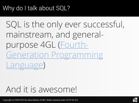
From early days onwards, programming language designers had this desire to design languages in which you tell the machine WHAT you want as a result, not HOW to obtain it. For instance, in SQL, you tell the machine that you want to “connect” (JOIN) the user table and the address table and find the users that live in Switzerland. You don’t care HOW the database will retrieve this information (e.g. should the users table be loaded first, or the address table? Should the two tables be joined in a nested loop or with a hashmap? Should all data be loaded in memory first and then filtered for Swiss users, or should we only load Swiss addresses in the first place? Etc.)

As with every abstraction, you will still need to know the basics of what’s going on behind the scenes in a database to help the database make the right decisions when you query it. For instance, it makes sense to:

• Establish a formal foreign key relationship between the tables (this tells the database that every address is guaranteed to have a corresponding user)
• Add an index on the search field: The country (this tells the database that specific countries can be found in O(log N) instead of O(N))

But once your database and your application matures, you will have put all the important meta data in place and you can focus on your business logic only. The following 10 tricks show amazing functionality written in only a few lines of declarative SQL, producing simple and also complex output.

1. Everything is a Table

This is the most trivial of tricks, and not even really a trick, but it is fundamental to a thorough understanding of SQL: Everything is a table! When you see a SQL statement like this:

SELECT *
FROM person

… you will quickly spot the table person sitting right there in the FROM clause. That’s cool, that is a table. But did you realise that the whole statement is also a table? For instance, you can write:

SELECT *
FROM (
  SELECT *
  FROM person
) t

And now, you have created what is called a “derived table” – i.e. a nested SELECT statement in a FROM clause.

That’s trivial, but if you think of it, quite elegant. You can also create ad-hoc, in-memory tables with the VALUES() constructor as such, in some databases (e.g. PostgreSQL, SQL Server):

SELECT *
FROM (
  VALUES(1),(2),(3)
) t(a)

Which simply yields:

a
---
 1
 2
 3

If that clause is not supported, you can revert to derived tables, e.g. in Oracle:

SELECT *
FROM (
  SELECT 1 AS a FROM DUAL UNION ALL
  SELECT 2 AS a FROM DUAL UNION ALL
  SELECT 3 AS a FROM DUAL
) t

Now that you’re seeing that VALUES() and derived tables are really the same thing, conceptually, let’s review the INSERT statement, which comes in two flavours:

-- SQL Server, PostgreSQL, some others:
INSERT INTO my_table(a)
VALUES(1),(2),(3);

-- Oracle, many others:
INSERT INTO my_table(a)
SELECT 1 AS a FROM DUAL UNION ALL
SELECT 2 AS a FROM DUAL UNION ALL
SELECT 3 AS a FROM DUAL

In SQL everything is a table. When you’re inserting rows into a table, you’re not really inserting individual rows. You’re really inserting entire tables. Most people just happen to insert a single-row-table most of the time, and thus don’t realise what INSERT really does.

Everything is a table. In PostgreSQL, even functions are tables:

SELECT *
FROM substring('abcde', 2, 3)

The above yields:

substring
---------
bcd

If you’re programming in Java, you can use the analogy of the Java 8 Stream API to take this one step further. Consider the following equivalent concepts:

TABLE          : Stream<Tuple<..>>
SELECT         : map() 
DISTINCT       : distinct()
JOIN           : flatMap()
WHERE / HAVING : filter()
GROUP BY       : collect()
ORDER BY       : sorted()
UNION ALL      : concat()

With Java 8, “everything is a Stream” (as soon as you start working with Streams, at least). No matter how you transform a stream, e.g. with map() or filter(), the resulting type is always a Stream again.

We’ve written an entire article to explain this more deeply, and to compare the Stream API with SQL: Common SQL Clauses and Their Equivalents in Java 8 Streams

And if you’re looking for “better streams” (i.e. streams with even more SQL semantics), do check out jOOλ, an open source library that brings SQL window functions to Java.

2. Data Generation with Recursive SQL

Common Table Expressions (also: CTE, also referred to as subquery factoring, e.g. in Oracle) are the only way to declare variables in SQL (apart from the obscure WINDOW clause that only PostgreSQL and Sybase SQL Anywhere know).

This is a powerful concept. Extremely powerful. Consider the following statement:

-- Table variables
WITH 
  t1(v1, v2) AS (SELECT 1, 2),
  t2(w1, w2) AS (
    SELECT v1 * 2, v2 * 2
    FROM t1
  )
SELECT *
FROM t1, t2

It yields

v1   v2   v3   v4
-----------------
 1    2    2    4

Using the simple WITH clause, you can specify a list of table variables (remember: everything is a table), which may even depend on each other.

That is easy to understand. This makes CTE (Common Table Expressions) already very useful, but what’s really really awesome is that they’re allowed to be recursive! Consider the following PostgreSQL example:

WITH RECURSIVE t(v) AS (
  SELECT 1     -- Seed Row
  UNION ALL
  SELECT v + 1 -- Recursion
  FROM t
)
SELECT v
FROM t
LIMIT 5

It yields

v
---
 1
 2
 3
 4
 5

How does it work? It’s relatively easy, once you see through the many keywords. You define a common table expression that has exactly two UNION ALL subqueries.

The first UNION ALL subquery is what I usually call the “seed row”. It “seeds” (initialises) the recursion. It can produce one or several rows on which we will recurse afterwards. Remember: everything is a table, so our recursion will happen on a whole table, not on an individual row/value.

The second UNION ALL subquery is where the recursion happens. If you look closely, you will observe that it selects from t. I.e. the second subquery is allowed to select from the very CTE that we’re about to declare. Recursively. It thus has also access to the column v, which is being declared by the CTE that already uses it.

In our example, we seed the recursion with the row (1), and then recurse by adding v + 1. The recursion is then stopped at the use-site by setting a LIMIT 5 (beware of potentially infinite recursions – just like with Java 8 Streams).

Side note: Turing completeness

Recursive CTE make SQL:1999 turing complete, which means that any program can be written in SQL! (if you’re crazy enough)

One impressive example that frequently shows up on blogs: The Mandelbrot Set, e.g. as displayed on http://explainextended.com/2013/12/31/happy-new-year-5/

WITH RECURSIVE q(r, i, rx, ix, g) AS (
  SELECT r::DOUBLE PRECISION * 0.02, i::DOUBLE PRECISION * 0.02, 
        .0::DOUBLE PRECISION      , .0::DOUBLE PRECISION, 0
  FROM generate_series(-60, 20) r, generate_series(-50, 50) i
  UNION ALL
  SELECT r, i, CASE WHEN abs(rx * rx + ix * ix) <= 2 THEN rx * rx - ix * ix END + r, 
               CASE WHEN abs(rx * rx + ix * ix) <= 2 THEN 2 * rx * ix END + i, g + 1
  FROM q
  WHERE rx IS NOT NULL AND g < 99
)
SELECT array_to_string(array_agg(s ORDER BY r), '')
FROM (
  SELECT i, r, substring(' .:-=+*#%@', max(g) / 10 + 1, 1) s
  FROM q
  GROUP BY i, r
) q
GROUP BY i
ORDER BY i

Run the above on PostgreSQL, and you’ll get something like

.-.:-.......==..*.=.::-@@@@@:::.:.@..*-.         =. 
                             ...=...=...::+%.@:@@@@@@@@@@@@@+*#=.=:+-.      ..-  
                             .:.:=::*....@@@@@@@@@@@@@@@@@@@@@@@@=@@.....::...:. 
                             ...*@@@@=.@:@@@@@@@@@@@@@@@@@@@@@@@@@@=.=....:...::.
                              .::@@@@@:-@@@@@@@@@@@@@@@@@@@@@@@@@@@@:@..-:@=*:::.
                              .-@@@@@-@@@@@@@@@@@@@@@@@@@@@@@@@@@@@@@@@.=@@@@=..:
                              ...@@@@@@@@@@@@@@@@@@@@@@@@@@@@@@@@@@@@@@:@@@@@:.. 
                             ....:-*@@@@@@@@@@@@@@@@@@@@@@@@@@@@@@@@@@@@@@@@@::  
                            .....@@@@@@@@@@@@@@@@@@@@@@@@@@@@@@@@@@@@@@@@@@@-..  
                          .....@@@@@@@@@@@@@@@@@@@@@@@@@@@@@@@@@@@@@@@@@@@-:...  
                         .--:+.@@@@@@@@@@@@@@@@@@@@@@@@@@@@@@@@@@@@@@@@@@@@@...  
                         .==@@@@@@@@@@@@@@@@@@@@@@@@@@@@@@@@@@@@@@@@@@@@@@@@-..  
                         ..+@@@@@@@@@@@@@@@@@@@@@@@@@@@@@@@@@@@@@@@@@@@@@@@@-#.  
                         ...=+@@@@@@@@@@@@@@@@@@@@@@@@@@@@@@@@@@@@@@@@@@@@@@@@.. 
                         -.=-@@@@@@@@@@@@@@@@@@@@@@@@@@@@@@@@@@@@@@@@@@@@@@@@@..:
                        .*%:@@@@@@@@@@@@@@@@@@@@@@@@@@@@@@@@@@@@@@@@@@@@@@@@@@:@-
 .    ..:...           ..-@@@@@@@@@@@@@@@@@@@@@@@@@@@@@@@@@@@@@@@@@@@@@@@@@@@@@@@
..............        ....-@@@@@@@@@@@@@@@@@@@@@@@@@@@@@@@@@@@@@@@@@@@@@@@@@@@%@=
.--.-.....-=.:..........::@@@@@@@@@@@@@@@@@@@@@@@@@@@@@@@@@@@@@@@@@@@@@@@@@@@@@..
..=:-....=@+..=.........@@@@@@@@@@@@@@@@@@@@@@@@@@@@@@@@@@@@@@@@@@@@@@@@@@@@@@@:.
.:+@@::@==@-*:%:+.......:@@@@@@@@@@@@@@@@@@@@@@@@@@@@@@@@@@@@@@@@@@@@@@@@@@@@@@@.
::@@@-@@@@@@@@@-:=.....:@@@@@@@@@@@@@@@@@@@@@@@@@@@@@@@@@@@@@@@@@@@@@@@@@@@@@@@@:
.:@@@@@@@@@@@@@@@=:.....%@@@@@@@@@@@@@@@@@@@@@@@@@@@@@@@@@@@@@@@@@@@@@@@@@@@@@@@@
.:@@@@@@@@@@@@@@@@@-...:@@@@@@@@@@@@@@@@@@@@@@@@@@@@@@@@@@@@@@@@@@@@@@@@@@@@@@@:-
:@@@@@@@@@@@@@@@@@@@-..%@@@@@@@@@@@@@@@@@@@@@@@@@@@@@@@@@@@@@@@@@@@@@@@@@@@@@@@@.
%@@@@@@@@@@@@@@@@@@@-..-@@@@@@@@@@@@@@@@@@@@@@@@@@@@@@@@@@@@@@@@@@@@@@@@@@@@@@@@.
@@@@@@@@@@@@@@@@@@@@@::+@@@@@@@@@@@@@@@@@@@@@@@@@@@@@@@@@@@@@@@@@@@@@@@@@@@@@@@@+
@@@@@@@@@@@@@@@@@@@@@@:@@@@@@@@@@@@@@@@@@@@@@@@@@@@@@@@@@@@@@@@@@@@@@@@@@@@@@@@..
@@@@@@@@@@@@@@@@@@@@@@-@@@@@@@@@@@@@@@@@@@@@@@@@@@@@@@@@@@@@@@@@@@@@@@@@@@@@@@@- 
@@@@@@@@@@@@@@@@@@@@@@@@@@@@@@@@@@@@@@@@@@@@@@@@@@@@@@@@@@@@@@@@@@@@@@@@@@@@@@.

Impressive, huh?

3. Running Total Calculations

This blog is full of running total examples. They’re some of the most educational examples to learn about advanced SQL, because there are at least a dozen of ways how to implement a running total.

A running total is easy to understand, conceptually.

In Microsoft Excel, you would simply calculate a sum (or difference) of two previous (or subsequent) values, and then use the useful crosshair cursor to pull that formula through your entire spreadsheet. You “run” that total through the spreadsheet. A “running total”.

In SQL, the best way to do that is by using window functions, another topic that this blog has covered many many times.

Window functions are a powerful concept – not so easy to understand at first, but in fact, they’re really really easy:

Window functions are aggregations / rankings on a subset of rows relative to the current row being transformed by SELECT

That’s it.

What it essentially means is that a window function can perform calculations on rows that are “above” or “below” the current row. Unlike ordinary aggregations and GROUP BY, however, they don’t transform the rows, which makes them very useful.

The syntax can be summarised as follows, with individual parts being optional

function(...) OVER (
  PARTITION BY ...
  ORDER BY ...
  ROWS BETWEEN ... AND ...
)

So, we have any sort of function (we’ll see examples for such functions later), followed by this OVER() clause, which specifies the window. I.e. this OVER() clause defines:

• The PARTITION: Only rows that are in the same partition as the current row will be considered for the window
• The ORDER: The window can be ordered independently of what we’re selecting
• The ROWS (or RANGE) frame definition: The window can be restricted to a fixed amount of rows “ahead” and “behind”

That’s all there is to window functions.

Now how does that help us calculate a running total? Consider the following data:

| ID   | VALUE_DATE | AMOUNT |    BALANCE |
|------|------------|--------|------------|
| 9997 | 2014-03-18 |  99.17 |   19985.81 |
| 9981 | 2014-03-16 |  71.44 |   19886.64 |
| 9979 | 2014-03-16 | -94.60 |   19815.20 |
| 9977 | 2014-03-16 |  -6.96 |   19909.80 |
| 9971 | 2014-03-15 | -65.95 |   19916.76 |

Let’s assume that BALANCE is what we want to calculate from AMOUNT

Intuitively, we can immediately see that the following holds true:

So, in plain English, any balance can be expressed with the following pseudo SQL:

TOP_BALANCE - SUM(AMOUNT) OVER (
  "all the rows on top of the current row"
)

In real SQL, that would then be written as follows:

SUM(t.amount) OVER (
  PARTITION BY t.account_id 
  ORDER BY     t.value_date DESC,
               t.id         DESC
  ROWS BETWEEN UNBOUNDED PRECEDING
       AND     1         PRECEDING
)

Explanation:

• The partition will calculate the sum for each bank account, not for the entire data set
• The ordering will guarantee that transactions are ordered (within the partition) prior to summing
• The rows clause will consider only preceding rows (within the partition, given the ordering) prior to summing

All of this will happen in-memory over the data set that has already been selected by you in your FROM .. WHERE etc. clauses, and is thus extremely fast.

Intermezzo

Before we move on to all the other awesome tricks, consider this: We’ve seen

• (Recursive) Common Table Expressions (CTE)
• Window functions

Both of these features are:

• Awesome
• Exremely powerful
• Declarative
• Part of the SQL standard
• Available in most popular RDBMS (except MySQL)
• Very important building blocks

If anything can be concluded from this article, it is the fact that you should absolutely know these two building blocks of modern SQL. Why? Because:

4. Finding the Largest Series with no Gaps

Stack Overflow has this very nice feature to motivate people to stay on their website for as long as possible. Badges:

For scale, you can see how many badges I have. Tons.

How do you calculate these badges? Let’s have a look at the “Enthusiast” and the “Fanatic”. These badges are awarded to anyone who spends a given amount of consecutive days on their platform. Regardless of any wedding date or wife’s birthday, you HAVE TO LOG IN, or the counter starts from zero again.

Now as we’re doing declarative programming, we don’t care about maintaining any state and in-memory counters. We want to express this in the form of online analytic SQL. I.e. consider this data:

| LOGIN_TIME          |
|---------------------|
| 2014-03-18 05:37:13 |
| 2014-03-16 08:31:47 |
| 2014-03-16 06:11:17 |
| 2014-03-16 05:59:33 |
| 2014-03-15 11:17:28 |
| 2014-03-15 10:00:11 |
| 2014-03-15 07:45:27 |
| 2014-03-15 07:42:19 |
| 2014-03-14 09:38:12 |

That doesn’t help much. Let’s remove the hours from the timestamp. That’s easy:

SELECT DISTINCT 
  cast(login_time AS DATE) AS login_date
FROM logins
WHERE user_id = :user_id

Which yields:

| LOGIN_DATE |
|------------|
| 2014-03-18 |
| 2014-03-16 |
| 2014-03-15 |
| 2014-03-14 |

Now, that we’ve learned about window functions, let’s just add a simple row number to each of these dates:

SELECT
  login_date,
  row_number() OVER (ORDER BY login_date)
FROM login_dates

Which produces:

| LOGIN_DATE | RN |
|------------|----|
| 2014-03-18 |  4 |
| 2014-03-16 |  3 |
| 2014-03-15 |  2 |
| 2014-03-14 |  1 |

Still easy. Now, what happens, if instead of selecting these values separately, we subtract them?

SELECT
  login_date -
  row_number() OVER (ORDER BY login_date)
FROM login_dates

We’re getting something like this:

| LOGIN_DATE | RN | GRP        |
|------------|----|------------|
| 2014-03-18 |  4 | 2014-03-14 |
| 2014-03-16 |  3 | 2014-03-13 |
| 2014-03-15 |  2 | 2014-03-13 |
| 2014-03-14 |  1 | 2014-03-13 |

Wow. Interesting. So, 14 - 1 = 13, 15 - 2 = 13, 16 - 3 = 13, but 18 - 4 = 14. No one can say it better than Doge:

There’s a simple example for this behaviour:

1. ROW_NUMBER() never has gaps. That’s how it’s defined
2. Our data, however, does

So when we subtract a “gapless” series of consecutive integers from a “gapful” series of non-consecutive dates, we will get the same date for each “gapless” subseries of consecutive dates, and we’ll get a new date again where the date series had gaps.

Huh.

This means we can now simply GROUP BY this arbitrary date value:

SELECT
  min(login_date), max(login_date),
  max(login_date) - 
  min(login_date) + 1 AS length
FROM login_date_groups
GROUP BY grp
ORDER BY length DESC

And we’re done. The largest series of consecutive dates with no gaps has been found:

| MIN        | MAX        | LENGTH |
|------------|------------|--------|
| 2014-03-14 | 2014-03-16 |      3 |
| 2014-03-18 | 2014-03-18 |      1 |

With the full query being:

WITH 
  login_dates AS (
    SELECT DISTINCT cast(login_time AS DATE) login_date 
    FROM logins WHERE user_id = :user_id
  ),
  login_date_groups AS (
    SELECT 
      login_date,
      login_date - row_number() OVER (ORDER BY login_date) AS grp
    FROM login_dates
  )
SELECT 
  min(login_date), max(login_date), 
  max(login_date) - min(login_date) + 1 AS length
FROM login_date_groups
GROUP BY grp
ORDER BY length DESC

Not that hard in the end, right? Of course, having the idea makes all the difference, but the query itself is really very very simple and elegant. No way you could implement some imperative-style algorithm in a leaner way than this.

Whew.

5. Finding the Length of a Series

Previously, we had seen series of consecutive values. That’s easy to deal with as we can abuse of the consecutiveness of integers. What if the definition of a “series” is less intuitive, and in addition to that, several series contain the same values? Consider the following data, where LENGTH is the length of each series that we want to calculate:

| ID   | VALUE_DATE | AMOUNT |     LENGTH |
|------|------------|--------|------------|
| 9997 | 2014-03-18 |  99.17 |          2 |
| 9981 | 2014-03-16 |  71.44 |          2 |
| 9979 | 2014-03-16 | -94.60 |          3 |
| 9977 | 2014-03-16 |  -6.96 |          3 |
| 9971 | 2014-03-15 | -65.95 |          3 |
| 9964 | 2014-03-15 |  15.13 |          2 |
| 9962 | 2014-03-15 |  17.47 |          2 |
| 9960 | 2014-03-15 |  -3.55 |          1 |
| 9959 | 2014-03-14 |  32.00 |          1 |

Yes, you’ve guessed right. A “series” is defined by the fact that consecutive (ordered by ID) rows have the same SIGN(AMOUNT). Check again the data formatted as below:

| ID   | VALUE_DATE | AMOUNT |     LENGTH |
|------|------------|--------|------------|
| 9997 | 2014-03-18 | +99.17 |          2 |
| 9981 | 2014-03-16 | +71.44 |          2 |

| 9979 | 2014-03-16 | -94.60 |          3 |
| 9977 | 2014-03-16 | - 6.96 |          3 |
| 9971 | 2014-03-15 | -65.95 |          3 |

| 9964 | 2014-03-15 | +15.13 |          2 |
| 9962 | 2014-03-15 | +17.47 |          2 |

| 9960 | 2014-03-15 | - 3.55 |          1 |

| 9959 | 2014-03-14 | +32.00 |          1 |

How do we do it? “Easy”�� First, let’s get rid of all the noise, and add another row number:

SELECT 
  id, amount,
  sign(amount) AS sign,
  row_number() 
    OVER (ORDER BY id DESC) AS rn
FROM trx

This will give us:

| ID   | AMOUNT | SIGN | RN |
|------|--------|------|----|
| 9997 |  99.17 |    1 |  1 |
| 9981 |  71.44 |    1 |  2 |

| 9979 | -94.60 |   -1 |  3 |
| 9977 |  -6.96 |   -1 |  4 |
| 9971 | -65.95 |   -1 |  5 |

| 9964 |  15.13 |    1 |  6 |
| 9962 |  17.47 |    1 |  7 |

| 9960 |  -3.55 |   -1 |  8 |

| 9959 |  32.00 |    1 |  9 |

Now, the next goal is to produce the following table:

| ID   | AMOUNT | SIGN | RN | LO | HI |
|------|--------|------|----|----|----|
| 9997 |  99.17 |    1 |  1 |  1 |    |
| 9981 |  71.44 |    1 |  2 |    |  2 |

| 9979 | -94.60 |   -1 |  3 |  3 |    |
| 9977 |  -6.96 |   -1 |  4 |    |    |
| 9971 | -65.95 |   -1 |  5 |    |  5 |

| 9964 |  15.13 |    1 |  6 |  6 |    |
| 9962 |  17.47 |    1 |  7 |    |  7 |

| 9960 |  -3.55 |   -1 |  8 |  8 |  8 |

| 9959 |  32.00 |    1 |  9 |  9 |  9 |

In this table, we want to copy the row number value into “LO” at the “lower” end of a series, and into “HI” at the “upper” end of a series. For this we’ll be using the magical LEAD() and LAG(). LEAD() can access the n-th next row from the current row, whereas LAG() can access the n-th previous row from the current row. For example:

SELECT 
  lag(v) OVER (ORDER BY v),
  v, 
  lead(v) OVER (ORDER BY v)
FROM (
  VALUES (1), (2), (3), (4)
) t(v)

The above query produces:

That’s awesome! Remember, with window functions, you can perform rankings or aggregations on a subset of rows relative to the current row. In the case of LEAD() and LAG(), we simply access a single row relative to the current row, given its offset. This is useful in so many cases.

Continuing with our “LO” and “HI” example, we can simply write:

SELECT 
  trx.*,
  CASE WHEN lag(sign) 
       OVER (ORDER BY id DESC) != sign 
       THEN rn END AS lo,
  CASE WHEN lead(sign) 
       OVER (ORDER BY id DESC) != sign 
       THEN rn END AS hi,
FROM trx

… in which we compare the “previous” sign (lag(sign)) with the “current” sign (sign). If they’re different, we put the row number in “LO”, because that’s the lower bound of our series.

Then we compare the “next” sign (lead(sign)) with the “current” sign (sign). If they’re different, we put the row number in “HI”, because that’s the upper bound of our series.

Finally, a little boring NULL handling to get everything right, and we’re done:

SELECT -- With NULL handling...
  trx.*,
  CASE WHEN coalesce(lag(sign) 
       OVER (ORDER BY id DESC), 0) != sign 
       THEN rn END AS lo,
  CASE WHEN coalesce(lead(sign) 
       OVER (ORDER BY id DESC), 0) != sign 
       THEN rn END AS hi,
FROM trx

Next step. We want “LO” and “HI” to appear in ALL rows, not just at the “lower” and “upper” bounds of a series. E.g. like this:

| ID   | AMOUNT | SIGN | RN | LO | HI |
|------|--------|------|----|----|----|
| 9997 |  99.17 |    1 |  1 |  1 |  2 |
| 9981 |  71.44 |    1 |  2 |  1 |  2 |

| 9979 | -94.60 |   -1 |  3 |  3 |  5 |
| 9977 |  -6.96 |   -1 |  4 |  3 |  5 |
| 9971 | -65.95 |   -1 |  5 |  3 |  5 |

| 9964 |  15.13 |    1 |  6 |  6 |  7 |
| 9962 |  17.47 |    1 |  7 |  6 |  7 |

| 9960 |  -3.55 |   -1 |  8 |  8 |  8 |

| 9959 |  32.00 |    1 |  9 |  9 |  9 |

We’re using a feature that is available at least in Redshift, Sybase SQL Anywhere, DB2, Oracle. We’re using the “IGNORE NULLS” clause that can be passed to some window functions:

SELECT 
  trx.*,
  last_value (lo) IGNORE NULLS OVER (
    ORDER BY id DESC 
    ROWS BETWEEN UNBOUNDED PRECEDING 
    AND CURRENT ROW) AS lo,
  first_value(hi) IGNORE NULLS OVER (
    ORDER BY id DESC 
    ROWS BETWEEN CURRENT ROW 
    AND UNBOUNDED FOLLOWING) AS hi
FROM trx

A lot of keywords! But the essence is always the same. From any given “current” row, we look at all the “previous values” (ROWS BETWEEN UNBOUNDED PRECEDING AND CURRENT ROW), but ignoring all the nulls. From those previous values, we take the last value, and that’s our new “LO” value. In other words, we take the “closest preceding” “LO” value.

The same with “HI”. From any given “current” row, we look at all the “subsequent values” (ROWS BETWEEN CURRENT ROW AND UNBOUNDED FOLLOWING), but ignoring all the nulls. From the subsequent values, we take the first value, and that’s our new “HI” value. In other words, we take the “closest following” “HI” value.

Explained in Powerpoint:

Getting it 100% correct, with a little boring NULL fiddling:

SELECT -- With NULL handling...
  trx.*,
  coalesce(last_value (lo) IGNORE NULLS OVER (
    ORDER BY id DESC 
    ROWS BETWEEN UNBOUNDED PRECEDING 
    AND CURRENT ROW), rn) AS lo,
  coalesce(first_value(hi) IGNORE NULLS OVER (
    ORDER BY id DESC 
    ROWS BETWEEN CURRENT ROW 
    AND UNBOUNDED FOLLOWING), rn) AS hi
FROM trx

Finally, we’re just doing a trivial last step, keeping in mind off-by-1 errors:

SELECT
  trx.*,
  1 + hi - lo AS length
FROM trx

And we’re done. Here’s our result:

| ID   | AMOUNT | SIGN | RN | LO | HI | LENGTH|
|------|--------|------|----|----|----|-------|
| 9997 |  99.17 |    1 |  1 |  1 |  2 |     2 |
| 9981 |  71.44 |    1 |  2 |  1 |  2 |     2 |
| 9979 | -94.60 |   -1 |  3 |  3 |  5 |     3 |
| 9977 |  -6.96 |   -1 |  4 |  3 |  5 |     3 |
| 9971 | -65.95 |   -1 |  5 |  3 |  5 |     3 |
| 9964 |  15.13 |    1 |  6 |  6 |  7 |     2 |
| 9962 |  17.47 |    1 |  7 |  6 |  7 |     2 |
| 9960 |  -3.55 |   -1 |  8 |  8 |  8 |     1 |
| 9959 |  32.00 |    1 |  9 |  9 |  9 |     1 |

And the full query here:

WITH 
  trx1(id, amount, sign, rn) AS (
    SELECT id, amount, sign(amount), row_number() OVER (ORDER BY id DESC)
    FROM trx
  ),
  trx2(id, amount, sign, rn, lo, hi) AS (
    SELECT trx1.*,
    CASE WHEN coalesce(lag(sign) OVER (ORDER BY id DESC), 0) != sign 
         THEN rn END,
    CASE WHEN coalesce(lead(sign) OVER (ORDER BY id DESC), 0) != sign 
         THEN rn END
    FROM trx1
  )
SELECT 
  trx2.*, 1
  - last_value (lo) IGNORE NULLS OVER (ORDER BY id DESC 
    ROWS BETWEEN UNBOUNDED PRECEDING AND CURRENT ROW)
  + first_value(hi) IGNORE NULLS OVER (ORDER BY id DESC 
    ROWS BETWEEN CURRENT ROW AND UNBOUNDED FOLLOWING)
FROM trx2

Huh. This SQL thing does start getting interesting!

Ready for more?

6. The subset sum problem with SQL

This is my favourite!

What is the subset sum problem? Find a fun explanation here:
https://xkcd.com/287

And a boring one here:
https://en.wikipedia.org/wiki/Subset_sum_problem

Essentially, for each of these totals…

| ID | TOTAL |
|----|-------|
|  1 | 25150 |
|  2 | 19800 |
|  3 | 27511 |

… we want to find the “best” (i.e. the closest) sum possible, consisting of any combination of these items:

| ID   |  ITEM |
|------|-------|
|    1 |  7120 |
|    2 |  8150 |
|    3 |  8255 |
|    4 |  9051 |
|    5 |  1220 |
|    6 | 12515 |
|    7 | 13555 |
|    8 |  5221 |
|    9 |   812 |
|   10 |  6562 |

As you’re all quick with your mental mathemagic processing, you have immediately calculated these to be the best sums:

| TOTAL |  BEST | CALCULATION
|-------|-------|--------------------------------
| 25150 | 25133 | 7120 + 8150 + 9051 + 812
| 19800 | 19768 | 1220 + 12515 + 5221 + 812
| 27511 | 27488 | 8150 + 8255 + 9051 + 1220 + 812

How to do it with SQL? Easy. Just create a CTE that contains all the 2ⁿ *possible* sums and then find the closest one for each TOTAL:

-- All the possible 2N sums
WITH sums(sum, max_id, calc) AS (...)

-- Find the best sum per “TOTAL”
SELECT 
  totals.total,
  something_something(total - sum) AS best,
  something_something(total - sum) AS calc
FROM draw_the_rest_of_the_*bleep*_owl

As you’re reading this, you might be like my friend here:

But don’t worry, the solution is – again – not all that hard (although it doesn’t perform due to the nature of the algorithm):

WITH sums(sum, id, calc) AS (
  SELECT item, id, to_char(item) FROM items
  UNION ALL
  SELECT item + sum, items.id, calc || ' + ' || item
  FROM sums JOIN items ON sums.id < items.id
)
SELECT 
  totals.id,
  totals.total,
  min (sum) KEEP (
    DENSE_RANK FIRST ORDER BY abs(total - sum)
  ) AS best,
  min (calc) KEEP (
    DENSE_RANK FIRST ORDER BY abs(total - sum)
  ) AS calc,
FROM totals 
CROSS JOIN sums
GROUP BY totals.id, totals.total

In this article, I won’t explain the details of this solution, because the example has been taken from a previous article that you can find here:

How to Find the Closest Subset Sum with SQL

Enjoy reading the details, but be sure to come back here for the remaining 4 tricks:

7. Capping a Running Total

So far, we’ve seen how to calculate an “ordinary” running total with SQL using window functions. That was easy. Now, how about if we cap the running total such that it never goes below zero? Essentially, we want to calculate this:

| DATE       | AMOUNT | TOTAL |
|------------|--------|-------|
| 2012-01-01 |    800 |   800 |
| 2012-02-01 |   1900 |  2700 |
| 2012-03-01 |   1750 |  4450 |
| 2012-04-01 | -20000 |     0 |
| 2012-05-01 |    900 |   900 |
| 2012-06-01 |   3900 |  4800 |
| 2012-07-01 |  -2600 |  2200 |
| 2012-08-01 |  -2600 |     0 |
| 2012-09-01 |   2100 |  2100 |
| 2012-10-01 |  -2400 |     0 |
| 2012-11-01 |   1100 |  1100 |
| 2012-12-01 |   1300 |  2400 |

So, when that big negative AMOUNT -20000 was subtracted, instead of displaying the real TOTAL of -15550, we simply display 0. In other words (or data sets):

| DATE       | AMOUNT | TOTAL |
|------------|--------|-------|
| 2012-01-01 |    800 |   800 | GREATEST(0,    800)
| 2012-02-01 |   1900 |  2700 | GREATEST(0,   2700)
| 2012-03-01 |   1750 |  4450 | GREATEST(0,   4450)
| 2012-04-01 | -20000 |     0 | GREATEST(0, -15550)
| 2012-05-01 |    900 |   900 | GREATEST(0,    900)
| 2012-06-01 |   3900 |  4800 | GREATEST(0,   4800)
| 2012-07-01 |  -2600 |  2200 | GREATEST(0,   2200)
| 2012-08-01 |  -2600 |     0 | GREATEST(0,   -400)
| 2012-09-01 |   2100 |  2100 | GREATEST(0,   2100)
| 2012-10-01 |  -2400 |     0 | GREATEST(0,   -300)
| 2012-11-01 |   1100 |  1100 | GREATEST(0,   1100)
| 2012-12-01 |   1300 |  2400 | GREATEST(0,   2400)

How will we do it?

Exactly. With obscure, vendor-specific SQL. In this case, we’re using Oracle SQL

How does it work? Surprisingly easy!

Just add MODEL after any table, and you’re opening up a can of awesome SQL worms!

SELECT ... FROM some_table

-- Put this after any table
MODEL ...

Once we put MODEL there, we can implement spreadsheet logic directly in our SQL statements, just as with Microsoft Excel.

The following three clauses are the most useful and widely used (i.e. 1-2 per year by anyone on this planet):

MODEL
  -- The spreadsheet dimensions
  DIMENSION BY ...
  
  -- The spreadsheet cell type
  MEASURES ...
  
  -- The spreadsheet formulas
  RULES ...

The meaning of each of these three additional clauses is best explained with slides again.

The DIMENSION BY clause specifies the dimensions of your spreadsheet. Unlike in MS Excel, you can have any number of dimensions in Oracle:

The MEASURES clause specifies the values that are available in each cell of your spreadsheet. Unlike in MS Excel, you can have a whole tuple in each cell in Oracle, not just a single value.

The RULES clause specifies the formulas that apply to each cell in your spreadsheet. Unlike in MS Excel, these rules / formulas are centralised at a single place, instead of being put inside of each cell:

This design makes MODEL a bit harder to use than MS Excel, but much more powerful, if you dare. The whole query will then be “trivially”:

SELECT *
FROM (
  SELECT date, amount, 0 AS total
  FROM amounts
)
MODEL 
  DIMENSION BY (row_number() OVER (ORDER BY date) AS rn)
  MEASURES (date, amount, total)
  RULES (
    total[any] = greatest(0,
	coalesce(total[cv(rn) - 1], 0) + amount[cv(rn)])
  )

This whole thing is so powerful, it ships with its own whitepaper by Oracle, so rather than explaining things further here in this article, please do read the excellent whitepaper:

• http://www.oracle.com/technetwork/middleware/bi-foundation/10gr1-twp-bi-dw-sqlmodel-131067.pdf

8. Time Series Pattern Recognition

If you’re into fraud detection or any other field that runs real time analytics on large data sets, time series pattern recognition is certainly not a new term to you.

If we review the “length of a series” data set, we might want to generate triggers on complex events over our time series as such:

|   ID | VALUE_DATE |  AMOUNT | LEN | TRIGGER
|------|------------|---------|-----|--------
| 9997 | 2014-03-18 | + 99.17 |   1 |
| 9981 | 2014-03-16 | - 71.44 |   4 |
| 9979 | 2014-03-16 | - 94.60 |   4 |      x
| 9977 | 2014-03-16 | -  6.96 |   4 |
| 9971 | 2014-03-15 | - 65.95 |   4 |
| 9964 | 2014-03-15 | + 15.13 |   3 |
| 9962 | 2014-03-15 | + 17.47 |   3 |
| 9960 | 2014-03-15 | +  3.55 |   3 |
| 9959 | 2014-03-14 | - 32.00 |   1 |

The rule of the above trigger is:

Trigger on the 3^rd repetition of an event if the event occurs more than 3 times.

Similar to the previous MODEL clause, we can do this with an Oracle-specific clause that was added to Oracle 12c:

SELECT ... FROM some_table

-- Put this after any table to pattern-match
-- the table’s contents
MATCH_RECOGNIZE (...)

The simplest possible application of MATCH_RECOGNIZE includes the following subclauses:

SELECT *
FROM series
MATCH_RECOGNIZE (
  -- Pattern matching is done in this order
  ORDER BY ...

  -- These are the columns produced by matches
  MEASURES ...

  -- A short specification of what rows are
  -- returned from each match
  ALL ROWS PER MATCH

  -- «Regular expressions» of events to match
  PATTERN (...)

  -- The definitions of «what is an event»
  DEFINE ...
)

That sounds crazy. Let’s look at some example clause implementations

SELECT *
FROM series
MATCH_RECOGNIZE (
  ORDER BY id
  MEASURES classifier() AS trg
  ALL ROWS PER MATCH
  PATTERN (S (R X R+)?)
  DEFINE
    R AS sign(R.amount) = prev(sign(R.amount)),
    X AS sign(X.amount) = prev(sign(X.amount))
)

What do we do here?

• We order the table by ID, which is the order in which we want to match events. Easy.
• We then specify the values that we want as a result. We want the “MEASURE” trg, which is defined as the classifier, i.e. the literal that we’ll use in the PATTERN afterwards. Plus we want all the rows from a match.
• We then specify a regular expression-like pattern. The pattern is an event “S” for Start, followed optionally by “R” for Repeat, “X” for our special event X, followed by one or more “R” for repeat again. If the whole pattern matches, we get SRXR or SRXRR or SRXRRR, i.e. X will be at the third position of a series of length >= 4
• Finally, we define R and X as being the same thing: The event when SIGN(AMOUNT) of the current row is the same as SIGN(AMOUNT) of the previous row. We don’t have to define “S”. “S” is just any other row.

This query will magically produce the following output:

|   ID | VALUE_DATE |  AMOUNT | TRG |
|------|------------|---------|-----|
| 9997 | 2014-03-18 | + 99.17 |   S |
| 9981 | 2014-03-16 | - 71.44 |   R |
| 9979 | 2014-03-16 | - 94.60 |   X |
| 9977 | 2014-03-16 | -  6.96 |   R |
| 9971 | 2014-03-15 | - 65.95 |   S |
| 9964 | 2014-03-15 | + 15.13 |   S |
| 9962 | 2014-03-15 | + 17.47 |   S |
| 9960 | 2014-03-15 | +  3.55 |   S |
| 9959 | 2014-03-14 | - 32.00 |   S |

We can see a single “X” in our event stream. Exactly where we had expected it. At the 3rd repetition of an event (same sign) in a series of length > 3.

Boom!

As we don’t really care about “S” and “R” events, let’s just remove them as such:

SELECT 
  id, value_date, amount, 
  CASE trg WHEN 'X' THEN 'X' END trg
FROM series
MATCH_RECOGNIZE (
  ORDER BY id
  MEASURES classifier() AS trg
  ALL ROWS PER MATCH
  PATTERN (S (R X R+)?)
  DEFINE
    R AS sign(R.amount) = prev(sign(R.amount)),
    X AS sign(X.amount) = prev(sign(X.amount))
)

to produce:

|   ID | VALUE_DATE |  AMOUNT | TRG |
|------|------------|---------|-----|
| 9997 | 2014-03-18 | + 99.17 |     |
| 9981 | 2014-03-16 | - 71.44 |     |
| 9979 | 2014-03-16 | - 94.60 |   X |
| 9977 | 2014-03-16 | -  6.96 |     |
| 9971 | 2014-03-15 | - 65.95 |     |
| 9964 | 2014-03-15 | + 15.13 |     |
| 9962 | 2014-03-15 | + 17.47 |     |
| 9960 | 2014-03-15 | +  3.55 |     |
| 9959 | 2014-03-14 | - 32.00 |     |

Thank you Oracle!

Again, don’t expect me to explain this any better than the excellent Oracle whitepaper already did, which I strongly recommend reading if you’re using Oracle 12c anyway:

• http://www.oracle.com/ocom/groups/public/@otn/documents/webcontent/1965433.pdf

9. Pivoting and Unpivoting

If you’ve read this far, the following will be almost too embarassingly simple:

This is our data, i.e. actors, film titles, and film ratings:

| NAME      | TITLE           | RATING |
|-----------|-----------------|--------|
| A. GRANT  | ANNIE IDENTITY  | G      |
| A. GRANT  | DISCIPLE MOTHER | PG     |
| A. GRANT  | GLORY TRACY     | PG-13  |
| A. HUDSON | LEGEND JEDI     | PG     |
| A. CRONYN | IRON MOON       | PG     |
| A. CRONYN | LADY STAGE      | PG     |
| B. WALKEN | SIEGE MADRE     | R      |

This is what we call pivoting:

| NAME      | NC-17 |  PG |   G | PG-13 |   R |
|-----------|-------|-----|-----|-------|-----|
| A. GRANT  |     3 |   6 |   5 |     3 |   1 |
| A. HUDSON |    12 |   4 |   7 |     9 |   2 |
| A. CRONYN |     6 |   9 |   2 |     6 |   4 |
| B. WALKEN |     8 |   8 |   4 |     7 |   3 |
| B. WILLIS |     5 |   5 |  14 |     3 |   6 |
| C. DENCH  |     6 |   4 |   5 |     4 |   5 |
| C. NEESON |     3 |   8 |   4 |     7 |   3 |

Observe how we kinda grouped by the actors and then “pivoted” the number films per rating each actor played in. Instead of displaying this in a “relational” way, (i.e. each group is a row) we pivoted the whole thing to produce a column per group. We can do this, because we know all the possible groups in advance.

Unpivoting is the opposite, when from the above, we want to get back to the “row per group” representation:

| NAME      | RATING | COUNT |
|-----------|--------|-------|
| A. GRANT  | NC-17  |     3 |
| A. GRANT  | PG     |     6 |
| A. GRANT  | G      |     5 |
| A. GRANT  | PG-13  |     3 |
| A. GRANT  | R      |     6 |
| A. HUDSON | NC-17  |    12 |
| A. HUDSON | PG     |     4 |

It’s actually really easy. This is how we’d do it in PostgreSQL:

SELECT 
  first_name, last_name,
  count(*) FILTER (WHERE rating = 'NC-17') AS "NC-17",
  count(*) FILTER (WHERE rating = 'PG'   ) AS "PG",
  count(*) FILTER (WHERE rating = 'G'    ) AS "G",
  count(*) FILTER (WHERE rating = 'PG-13') AS "PG-13",
  count(*) FILTER (WHERE rating = 'R'    ) AS "R"
FROM actor AS a
JOIN film_actor AS fa USING (actor_id)
JOIN film AS f USING (film_id)
GROUP BY actor_id

We can append a simple FILTER clause to an aggregate function in order to count only some of the data.

In all other databases, we’d do it like this:

SELECT 
  first_name, last_name,
  count(CASE rating WHEN 'NC-17' THEN 1 END) AS "NC-17",
  count(CASE rating WHEN 'PG'    THEN 1 END) AS "PG",
  count(CASE rating WHEN 'G'     THEN 1 END) AS "G",
  count(CASE rating WHEN 'PG-13' THEN 1 END) AS "PG-13",
  count(CASE rating WHEN 'R'     THEN 1 END) AS "R"
FROM actor AS a
JOIN film_actor AS fa USING (actor_id)
JOIN film AS f USING (film_id)
GROUP BY actor_id

The nice thing here is that aggregate functions usually only consider non-NULL values, so if we make all the values NULL that are not interesting per aggregation, we’ll get the same result.

Now, if you’re using either SQL Server, or Oracle, you can use the built-in PIVOT or UNPIVOT clauses instead. Again, as with MODEL or MATCH_RECOGNIZE, just append this new keyword after a table and get the same result:

-- PIVOTING
SELECT something, something
FROM some_table
PIVOT (
  count(*) FOR rating IN (
    'NC-17' AS "NC-17", 
    'PG'    AS "PG", 
    'G'     AS "G", 
    'PG-13' AS "PG-13", 
    'R'     AS "R"
  )
)

-- UNPIVOTING
SELECT something, something
FROM some_table
UNPIVOT (
  count    FOR rating IN (
    "NC-17" AS 'NC-17', 
    "PG"    AS 'PG', 
    "G"     AS 'G', 
    "PG-13" AS 'PG-13', 
    "R"     AS 'R'
  )
)

Easy. Next.

10. Abusing XML and JSON

First off

JSON is just XML with less features and less syntax

Now, everyone knows that XML is awesome. The corollary is thus:

JSON is less awesome

Don’t use JSON.

Now that we’ve settled this, we can safely ignore the ongoing JSON-in-the-database-hype (which most of you will regret in five years anyway), and move on to the final example. How to do XML in the database.

This is what we want to do:

Given the original XML document, we want to parse that document, unnest the comma-separated list of films per actor, and produce a denormalised representation of actors/films in a single relation.

Ready. Set. Go. This is the idea. We have three CTE:

WITH RECURSIVE
  x(v) AS (SELECT '...'::xml),
  actors(
    actor_id, first_name, last_name, films
  ) AS (...),
  films(
    actor_id, first_name, last_name, 
    film_id, film
  ) AS (...)
SELECT * 
FROM films

In the first one, we simply parse the XML. Here with PostgreSQL:

WITH RECURSIVE
  x(v) AS (SELECT '
<actors>
  <actor>
    <first-name>Bud</first-name>
    <last-name>Spencer</last-name>
    <films>God Forgives... I Don’t, Double Trouble, They Call Him Bulldozer</films>
  </actor>
  <actor>
    <first-name>Terence</first-name>
    <last-name>Hill</last-name>
    <films>God Forgives... I Don’t, Double Trouble, Lucky Luke</films>
  </actor>
</actors>'::xml),
  actors(actor_id, first_name, last_name, films) AS (...),
  films(actor_id, first_name, last_name, film_id, film) AS (...)
SELECT * 
FROM films

Easy.

Then, we do some XPath magic to extract the individual values from the XML structure and put those into columns:

WITH RECURSIVE
  x(v) AS (SELECT '...'::xml),
  actors(actor_id, first_name, last_name, films) AS (
    SELECT
      row_number() OVER (),
      (xpath('//first-name/text()', t.v))[1]::TEXT,
      (xpath('//last-name/text()' , t.v))[1]::TEXT,
      (xpath('//films/text()'     , t.v))[1]::TEXT
    FROM unnest(xpath('//actor', (SELECT v FROM x))) t(v)
  ),
  films(actor_id, first_name, last_name, film_id, film) AS (...)
SELECT * 
FROM films

Still easy.

Finally, just a bit of recursive regular expression pattern matching magic, and we’re done!

WITH RECURSIVE
  x(v) AS (SELECT '...'::xml),
  actors(actor_id, first_name, last_name, films) AS (...),
  films(actor_id, first_name, last_name, film_id, film) AS (
    SELECT actor_id, first_name, last_name, 1, 
      regexp_replace(films, ',.+', '')
    FROM actors
    UNION ALL
    SELECT actor_id, a.first_name, a.last_name, f.film_id + 1,
      regexp_replace(a.films, '.*' || f.film || ', ?(.*?)(,.+)?', '\1')
    FROM films AS f 
    JOIN actors AS a USING (actor_id)
    WHERE a.films NOT LIKE '%' || f.film
  )
SELECT * 
FROM films

Let’s conclude:

Conclusion

All of what this article has shown was declarative. And relatively easy. Of course, for the fun effect that I’m trying to achieve in this talk, some exaggerated SQL was taken and I expressly called everything “easy”. It’s not at all easy, you have to practice SQL. Like many other languages, but a bit harder because:

1. The syntax is a bit awkward from time to time
2. Declarative thinking is not easy. At least, it’s very different

But once you get a hang of it, declarative programming with SQL is totally worth it as you can express complex relationships between your data in very very little code by just describing the result you want to get from the database.

Isn’t that awesome?

And if that was a bit over the top, do note that I’m happy to visit your JUG / conference to give this talk (just contact us), or if you want to get really down into the details of these things, we also offer this talk as a public or in-house workshop. Do get in touch! We’re looking forward.

See again the full set of slides here:

Do you want to know how to develop your skillset to become a Java Rockstar?

Subscribe to our newsletter to start Rocking right now!

To get you started we give you our best selling eBooks for FREE!

1. JPA Mini Book

2. JVM Troubleshooting Guide

3. JUnit Tutorial for Unit Testing

4. Java Annotations Tutorial

5. Java Interview Questions

6. Spring Interview Questions

7. Android UI Design

and many more ....

I agree to the Terms and Privacy Policy

Sign up

Thank you!

We will contact you soon.