What is Layer Normalization?

Layer Normalization (LayerNorm) is a normalization technique used in neural networks to stabilize the distribution of activations during training. It computes the mean and variance across the feature dimensions of each individual input rather than across a batch, making it useful for architectures such as Transformers and recurrent neural networks.

Working

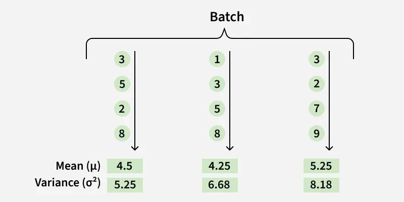
Consider an example where we have three vectors:

1. x_1 = [3.0, 5.0, 2.0, 8.0]
2. x_2 = [1.0, 3.0, 5.0, 8.0]
3. x_3 = [3.0, 2.0, 7.0, 9.0]

For each input x of the layer, Layer Normalization computes the following:

1. Mean & Variance for Each Feature

Mean and variance are calculated for each input but instead of across the batch, it’s done for the features (i.e per data point):

\mu = \frac{1}{H} \sum_{i=1}^{H} x_i

\sigma^2 = \frac{1}{H} \sum_{i=1}^{H} (x_i - \mu)^2

where:

• H is the number of features (neurons) in the layer
• x_i​ is the input for each feature
• \mu and \sigma^2 are the computed mean and variance.

Now, let's compute Mean and Variance for each feature (Per Data Point). For x_1 = [3.0, 5.0, 2.0, 8.0]:

1. Mean (\mu_1): \mu_1 = \frac{1}{4} (3.0 + 5.0 + 2.0 + 8.0) = \frac{18.0}{4} = 4.5
2. Variance (\sigma_1^2​): \sigma_1^2 = \frac{1}{4} \left[ (3.0 - 4.5)^2 + (5.0 - 4.5)^2 + (2.0 - 4.5)^2 + (8.0 - 4.5)^2 \right] = \frac{21.0}{4} = 5.25

Similarly compute for x_2 and x_3:

2. Normalize Input

Each feature is then normalized using the formula:

\hat{x}_i = \frac{x_i - \mu}{\sqrt{\sigma^2 + \epsilon}}

• Here \epsilon is a small constant added for numerical stability.

Now, we will normalize each feature in each vector by subtracting the mean and dividing by the standard deviation (square root of the variance) with a small constant \epsilon = 1e-5 added for numerical stability.

For x_1 = [3.0, 5.0, 2.0, 8.0]:

x_1' = \left[ \frac{3.0 - 4.5}{\sqrt{5.25 + 1e-5}}, \frac{5.0 - 4.5}{\sqrt{5.25 + 1e-5}}, \frac{2.0 - 4.5}{\sqrt{5.25 + 1e-5}}, \frac{8.0 - 4.5}{\sqrt{5.25 + 1e-5}} \right]

We calculate each normalized value for x_1​:

x_1' = [−0.6547,0.2182,−1.0911,1.5275]

For x_2 = [1.0, 3.0, 5.0, 8.0]:

x_2' = \left[ \frac{1.0 - 4.25}{\sqrt{8.3125 + 1e-5}}, \frac{3.0 - 4.25}{\sqrt{8.3125 + 1e-5}}, \frac{5.0 - 4.25}{\sqrt{8.3125 + 1e-5}}, \frac{8.0 - 4.25}{\sqrt{8.3125 + 1e-5}} \right]

We calculate each normalized value for x_2:

x_2' = [−1.2568,−0.4834,0.2900,1.4501]

For x_3 = [3.0, 2.0, 7.0, 9.0]:

x_3' = \left[ \frac{3.0 - 5.25}{\sqrt{3.6875 + 1e-5}}, \frac{2.0 - 5.25}{\sqrt{3.6875 + 1e-5}}, \frac{7.0 - 5.25}{\sqrt{3.6875 + 1e-5}}, \frac{9.0 - 5.25}{\sqrt{3.6875 + 1e-5}} \right]

We calculate each normalized value for x_3:

x_3' =[−0.7863,−1.1358,0.6116,1.3106]

3. Apply Scaling & Shifting

To ensure that the normalized activations can still represent a wide range of values, learnable parameters \gamma (scaling) and \beta (shifting) are introduced. Final output y is computed as:

y_i = \gamma \hat{x}_i + \beta

• This allows the network to scale and shift the normalized activations during training.

\gamma is the learnable scale parameter and \beta is the learnable shift parameter. Each feature has its own \gamma and \beta value.

\gamma \in \mathbb{R}^H

\beta \in \mathbb{R}^H

For simplicity, the following example uses scalar \gamma and \beta only to show the calculation steps. Here let’s assume \gamma = 1.5 and \beta = 0.5. We can apply this scaling and shifting to the normalized values to get the final output for each vector.

For x_1​: y_1 = [-0.4820, 0.8273, -1.1366, 2.7913]

For x_2​: y_2 = [-1.3851, -0.2250, 0.9350, 2.6751]

For x_3​: y_3 = [-0.6795, -1.2037, 1.4174, 2.4658]

These are the exact normalized values and the final outputs after applying Layer Normalization. For each individual input, LayerNorm computes the mean and variance across its feature dimensions.

Implementation in a Simple Neural Network with PyTorch

• nn.Linear(input_size, output_size): Creates a fully connected layer with the specified input and output dimensions.
• nn.LayerNorm(128): Applies Layer Normalization on the input of size 128.
• forward(self, x): Defines forward pass for the model by applying transformations to the input x step by step.
• torch.randn(10, 64): Generates a tensor of size (10, 64) filled with random values from a normal distribution.
• torch.relu(x): Applies ReLU (Rectified Linear Unit) activation function element-wise to x.

import torch
import torch.nn as nn

class SimpleNN(nn.Module):
    def __init__(self, input_size, output_size):
        super(SimpleNN, self).__init__()
        self.fc1 = nn.Linear(input_size, 128)
        self.layer_norm = nn.LayerNorm(128)  
        self.fc2 = nn.Linear(128, output_size)

    def forward(self, x):
        x = self.fc1(x)
        x = self.layer_norm(x) 
        x = torch.relu(x)
        x = self.fc2(x)
        return x

input_data = torch.randn(10, 64)
model = SimpleNN(64, 10)
output = model(input_data)
print(output)

Output:

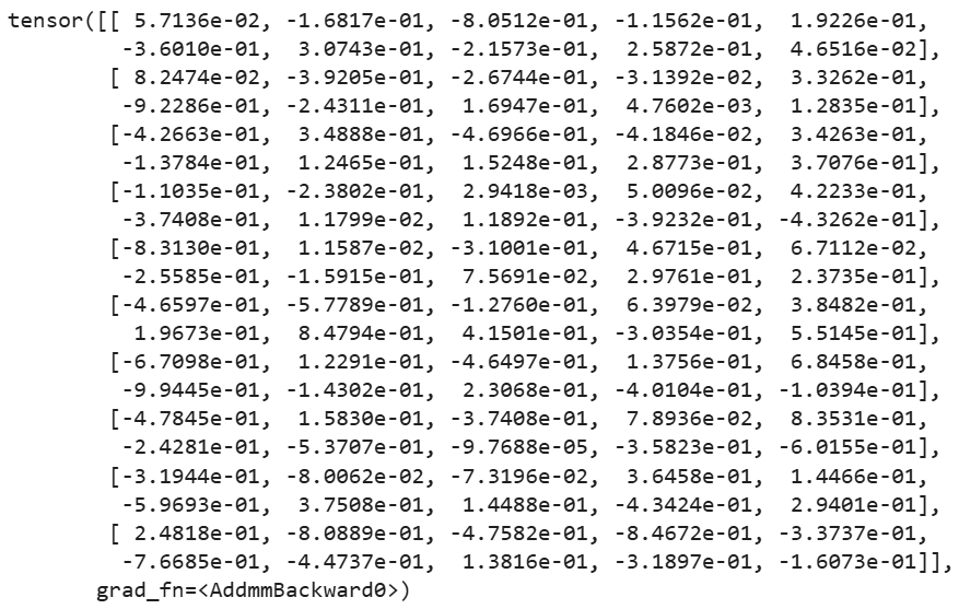
nn.LayerNorm(128) normalizes the 128 features of each input sample independently.

Advantages

1. Independent of batch size: It computes statistics for each sample, making it suitable for small or variable batch sizes.
2. Training stability: Normalizing activations can help maintain stable activation and gradient scales.
3. Useful for sequential models: It works well with models where batch statistics may be inconvenient, such as RNNs and Transformers.
4. Consistent behavior across samples: Each sample is normalized independently rather than relying on other samples in the batch.

Limitations

1. May not be ideal for every architecture: The effectiveness of LayerNorm depends on the model architecture and task.
2. Normalization can affect feature statistics: Normalizing feature activations may remove some information about their original scale.
3. Computational overhead: Although relatively inexpensive, normalization adds additional operations and learnable parameters.
4. Not a universal replacement for BatchNorm: BatchNorm can be more effective for some architectures, particularly conventional convolutional networks.

Layer Normalization vs Batch Normalization